Zernike Calculations in Julia

In optics, Zernike polynomials play a big role, and in many computer simulations of optical problems, it’s very important to be able to calculate their values on a polar or Cartesian grid. While this problem seems trivial (the exact formulae for Zernike polynomials are known) and is often used as MSc student assignment, it might become challenging for higher degrees of the polynomials due to their fast oscillating nature.

Recently, a fast and robust method of calculation of the Zernike polynomials and their derivatives in Cartesian coordinates was published [1]. I decided to give it a try and to program it in Julia, as the existing Julia’s implementations were not so far from the MSc student’s homework versions and are quite slow.

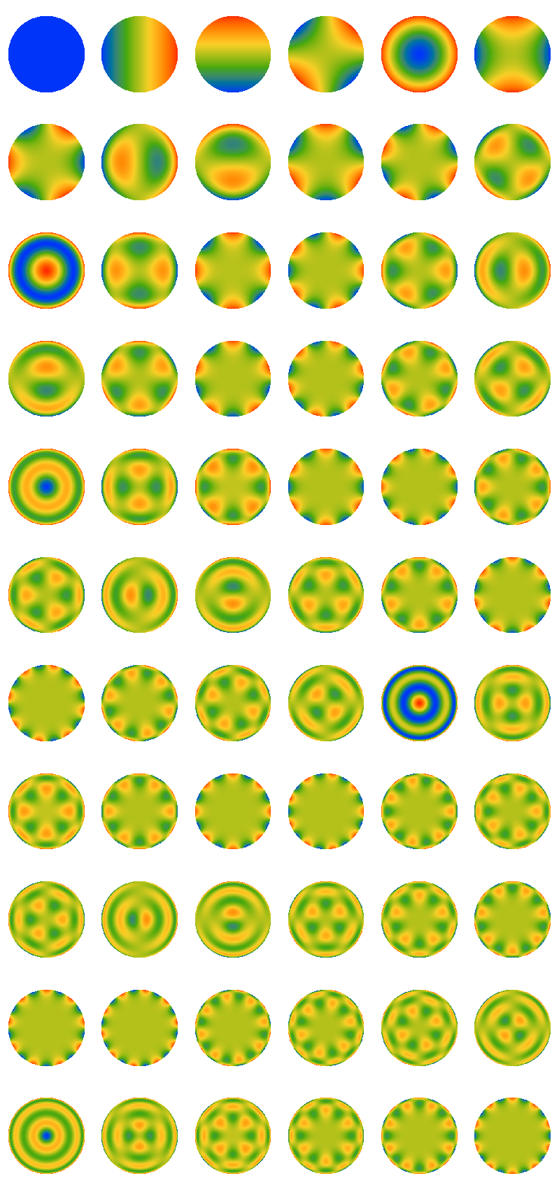
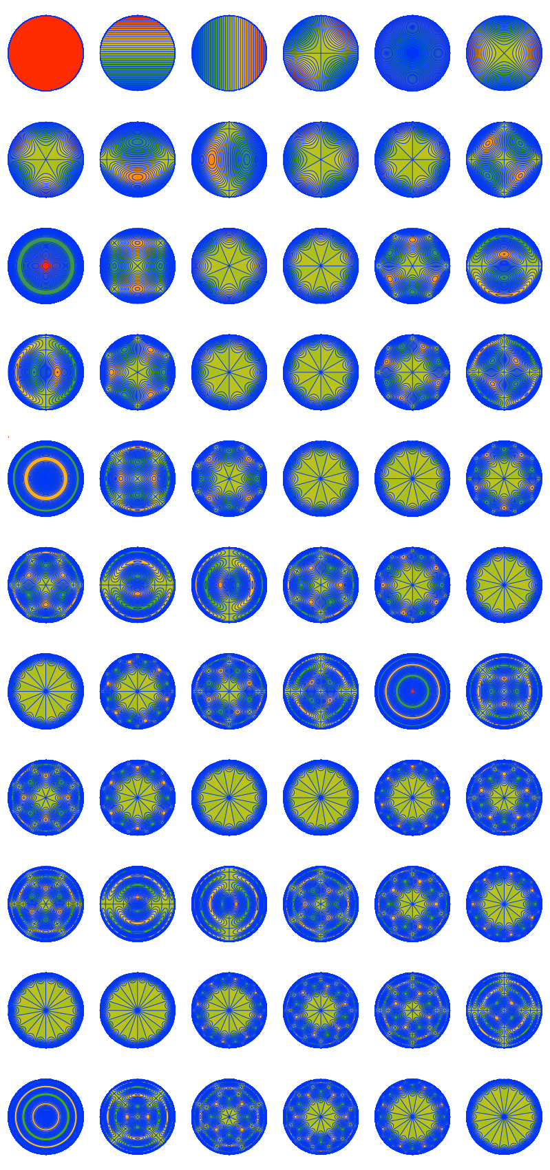
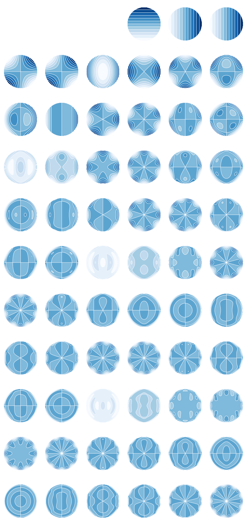
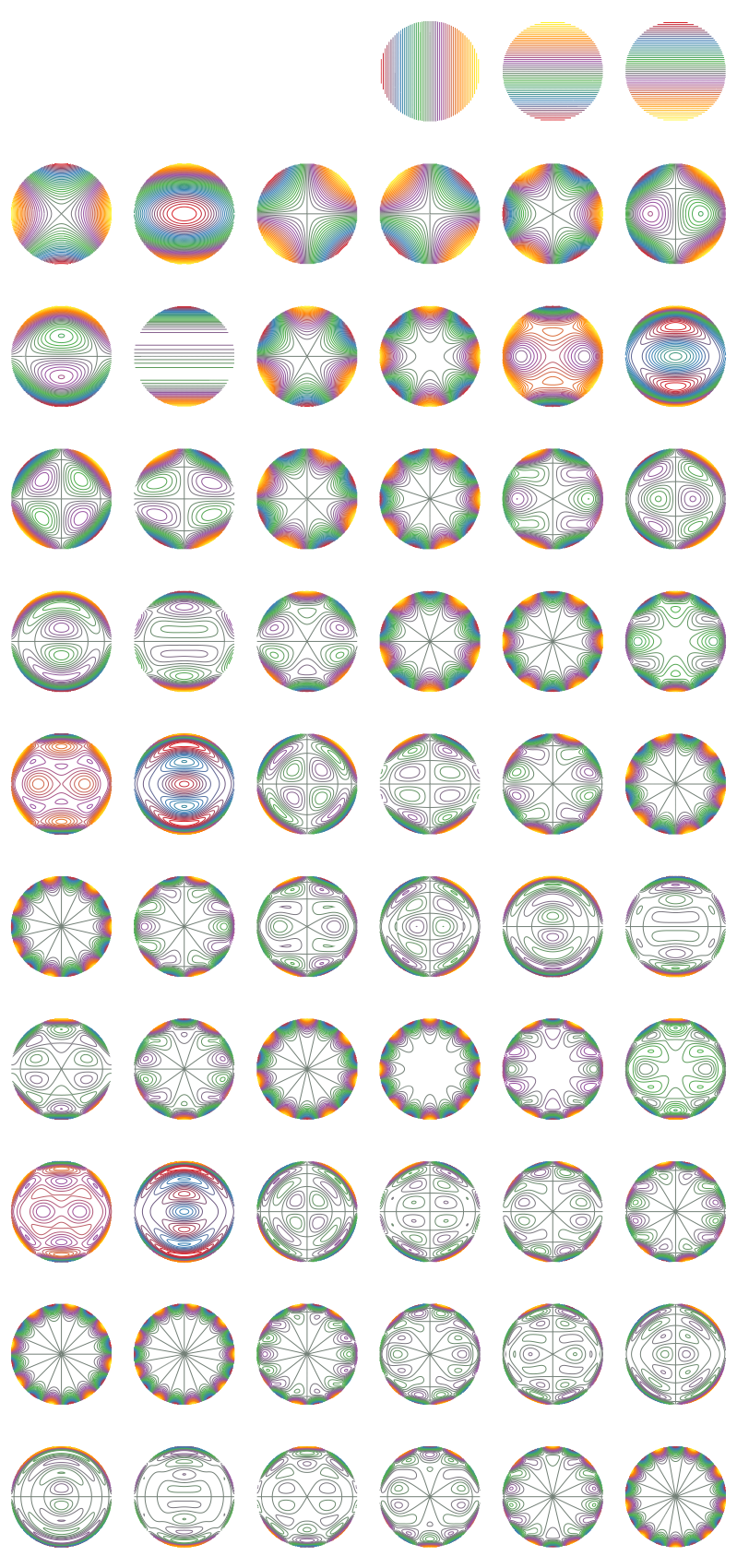
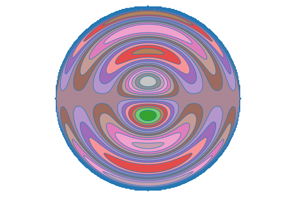
It was indeed really easy to translate the published pseudo-code in Julia. The implementation appeared to be indeed very fast, so I could not resist to play with some visualisations.

If you have Julia and Pluto installed, you can test the Zernike generation on your computer by downloading this Pluto notebook.

Alternatively, if you just want to play with the visualisations, you can use online Julia installation (warning: it will take some minutes to initialise, but then it runs quickly). For this, go to this page: http://pluto-on-binder.glitch.me/ and enter this link in the input box https://gist.github.com/olejorik/211e9a8763dc8e4508ba6f13dd939aca. The page will generate link to a virtual machine running my notebook with interactive Zernike calculations. You can change the notebooks inputs (use Shift+Enter to update the cells).

[1] T. B. Andersen, “Efficient and robust recurrence relations for the Zernike circle polynomials and their derivatives in Cartesian coordinates,” Opt. Express, vol. 26, no. 15, p. 18878, Jul. 2018